[WIP] Introduction to Algorithms

Chapter 1: The Role of Algorithms in Computing

A computational problem is a specification of a desired input-output relationship. e.g.

Computational problem: Sorting

Input: A sequence of $n$ values $(a_1$, ..., $a_n)$.

Output: A permutation (reordering) of the input such that $a'_1 \leq a'_2$ ... $a'_{n-1} \leq a'_n$.

An instance of a problem is all the inputs needed to compute a solution to the problem. Alternatively, a computational problem is the set of all (problem) instances and the desired output. e.g.

To sort the permutation {8, 3, 6, 7} is an instance of the general sorting problem and {3, 6, 7, 8} is the desired output.

An algorithm is a well-defined computational procedure that takes some input and produces an output in finite amount of time (i.e. it halts). A correct algorithm solves a computational problem by transforming to input into the desired output.

A data structure is a way to store and organize data in order to facilitate access and modifications.

Chapter 2: Getting Started

Objective: This chapter introduces the analysis of algorithms and algorithm design techniques like the incremental method (using insertion sort) and design-and-conquer (using merge sort).

Loop invariants

A loop invariant is a property or condition that holds true before and after every iteration of a loop. It is a useful tool for understanding the correctness of an algorithm.

It consists of three parts:

1. Initialization: Prove that the invariant is true before the first iteration.
2. Maintenance: Prove that if the invariant is true before an iteration, it remains true before the next iteration.
3. Termination: At the end of the loop, the invariant along with the termination condition should imply the correctness of the algorithm.

Insertion Sort

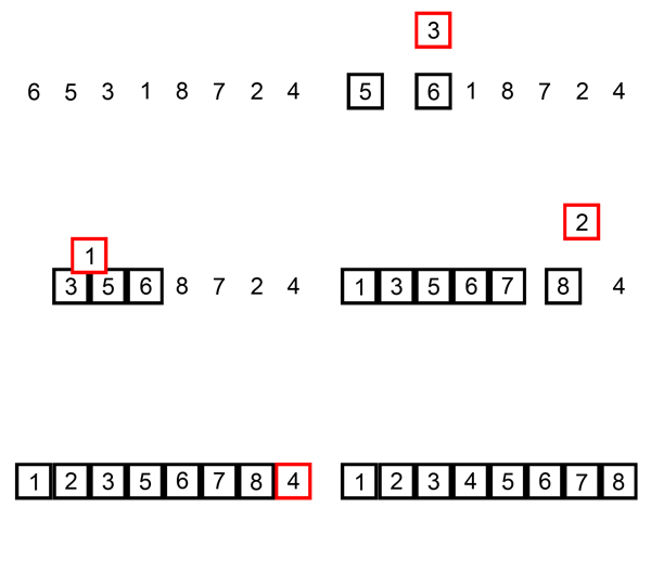
Insertion sort is a sorting algorithm that builds the final sorted array one item at a time. At each iteration, insertion sort removes one element from the input data, finds the location it belongs within the sorted list, and inserts it there. It repeats until no input elements remain.

fn insertion_sort(mut input: Vec<i32>) -> Vec<i32> {
    for i in 1..input.len() {
        let current = input[i];
        let mut j = i;

        while j > 0 && input[j - 1] > current {
            input[j] = input[j - 1];
            j -= 1;
        }

        input[j] = current;
    }

    input
}

Correctness of the insertion sort algorithm can be proven using loop invariants:

Invariant: At the start of each iteration, the sub-array input[0:i-1] contains the same elements as the original sub-array input[0:i-1], but in sorted order.

Proof:

• Initialization: Before the first iteration, $i = 1$. The sub-array input[0..i-1] (an empty subarray) is trivially sorted.
• Maintenance: The body of the for loop works by moving the elements in input[i - 1], input[i - 2], input[i - 3], ..., input[0] that are greater than input[i] one position to the right. This makes space for input[i] to be inserted in the correct position. The i variable is incremented and the sub-array input[0..i-1] is still sorted.
• Termination: The loop terminates when i = n. At this point, the sub-array input[0..n-1] is sorted and the algorithm has finished.

Exercises

2.1-1

• [31, 41, 59, 26, 41, 58] (i = 1, current = 41, j = 1)

• [31, 41, 59, 26, 41, 58] (i = 2, current = 59, j = 2)

• [31, 41, 59, 26, 41, 58] (i = 3, current = 26, j = 3)

• [31, 41, 59, 59, 41, 58] (i = 3, current = 26, j = 2)

• [31, 41, 41, 59, 41, 58] (i = 3, current = 26, j = 1)

• [31, 31, 41, 59, 41, 58] (i = 3, current = 26, j = 0)

• [26, 31, 41, 59, 41, 58] (i = 3, current = 26, j = 0)

• [26, 31, 41, 59, 41, 58] (i = 4, current = 41, j = 4)

• [26, 31, 41, 59, 59, 58] (i = 4, current = 41, j = 3)

• [26, 31, 41, 41, 59, 58] (i = 4, current = 41, j = 2)

• [26, 31, 41, 41, 59, 58] (i = 5, current = 58, j = 5)

• [26, 31, 41, 41, 59, 59] (i = 5, current = 58, j = 4)

• [26, 31, 41, 41, 58, 59] (i = 5, current = 58, j = 4)

2.1-2

Loop invariant: At the start of each iteration, the sum variable holds the sum of the first i-1 elements of the array.

Proof:

• Initialization: Before the first iteration, i = 0. The sum of all elements in input[0..(i-1)] is trivially zero because that sub-array contains no elements.
• Maintenance: The body of the for loop adds input[i] to the sum. The i variable is incremented and the sum is still the sum of all elements in input[0..(i-1)].
• Termination: When the loop terminates, i = n. sum is the sum of all elements in input[0..(i-1)] which equals input[0..(n-1)], which is all the elements in input.

2.1-3

fn insertion_sort_desc(mut input: Vec<i32>) -> Vec<i32> {
    for i in 1..input.len() {
        let current = input[i];
        let mut j = i;

        while j > 0 && input[j - 1] < current {
            input[j] = input[j - 1];
            j -= 1;
        }

        input[j] = current;
    }

    input
}

2.1-4

fn linear_search(input: Vec<i32>, needle: i32) -> Option<usize> {
    let mut result = Option::None;

    for i in 0..input.len() {
        let number = input[i];

        if number == needle {
            result = Option::Some(i);
            break;
        }
    }

    result
}

Loop invariant: At the start of each iteration, the result variable holds any element in input[0..(i-1)] that equals needle (or empty if none matches).

Proof:

• Initialization: Before the first iteration, i = 0. There are no elements in input[0..(i-1)], hence, result is empty.
• Maintenance: The body of the for loop sets result equal to input[i] if input[i] equals needle. The i variable is incremented and the result variable holds any element in input[0..(i-1)] that equals needle
• Termination: The loop terminates when i = n or when a match is found. In either, case the result variable holds any element in input[0..(i-1)] that equals needle (or empty if none matches).

2.1-5

fn add_binary_integers(a: Vec<u8>, b: Vec<u8>) -> Vec<u8> {
    if (a.len() != b.len()) {
        panic!("Both a and b must have the same length")
    }

    let mut result = vec![0; a.len() + 1];
    let mut overflow: u8 = 0;

    for i in (0..a.len()).rev() {
        let bit_sum = a[i] + b[i] + overflow;
        result[i+1] = bit_sum % 2;
        overflow = if bit_sum >= 2 { 1 } else { 0 }
    }

    result[0] = overflow;
    result
}

Analyzing algorithms

Analyzing an algorithm has come to mean predicting the resources that the algorithm requires. Resources include (but not limited to):

• Computational time
• Memory
• Communication bandwidth
• Energy consumption

To analyze algorithms, we need a model of the machine that it runs on, including the resources of that machine and a way to express their costs.

A common model is the random-access machine (RAM), which is a one-processor machine with the following properties:

• Instructions execute one after the other.
• Each primitive instruction takes a constant amount of time.
• Primitive instructions include:
  • Arithmetic operations,
  • Data access (i.e. reading or writing to memory)
  • Control operations (e.g. conditional and unconditional branch, subroutine call). Note: Calling a subroutine takes constant time, whereas executing the subroutine might not.

While simple, the RAM-model analyses are usually excellent predictors of performance on actual machines.

Why not empirical analysis?

One way to analyze an algorithm is to run it on a particular computer given a specific input. However, the result of this type of analysis depends on variables that are not inherent to the algorithm like computer type, current resource utilization, etc. Hence, you can't simply extrapolate this data and use it to compare different algorithms generally.

Analysis with the RAM model

A better form of analysis inspects features that are inherent to the algorithm and its input:

• The running time of an algorithm on a particular input is the number of primitive instructions executed on the RAM.
• An instruction that takes $c_k$ steps to execute and that executes $m$ times contributes $m \cdot c_k$ to the total running time.
• The running time of an algorithm is a function of its input.
• There are many features of the input that can affect an algorithm's running time. It's typical to only consider the input size due to its dominant effect.
• The best notion for input size depends on the problem being studied:
  • For problems like searching or sorting, the natural measure is the number of items in the input.
  • For problems like multiplication, the measure can be the total number of bits.
  • For some graph problems, it might be appropriate to describe the size of the input with more than one number (e.g. for the number of vertices and edges).
• Even for inputs of a given size, an algorithm can have different best-case and worst-case running times.

Analyzing insertion sort

fn insertion_sort(mut input: Vec<i32>) -> Vec<i32> {
    for i in 1..input.len() { // Line 1
        let current = input[i]; // Line 2
        let mut j = i; // Line 3

        while j > 0 && input[j - 1] > current { // Line 4
            input[j] = input[j - 1]; // Line 5
            j -= 1; // Line 6
        }

        input[j] = current; // Line 7
    }

    input // Line 8
}

For each i = 1, 2, ..., n, let $t_i$ denote the number of times the while loop test in line 4 is executed for that value of i. Empty lines are ignored as we assume they take no time.

For insertion sort on input of size $n$ , the best-case runtime happens when the input is already sorted. In this case, the while loop condition is checked and the loop is immediately terminated. Hence, $t_i = 1$ in this case for all $i$. The best-case runtime is then given by:

The best-case runtime is a linear function of $n$ because it can be expressed as $an + b$, where $a$ and $b$ are the various constants of running the instructions on the various lines.

For insertion sort, the worst case arises when the input is in reverse sorted order. In this case, the while loop is executed for all elements in input[0..(i-1)]. Hence, $t_i = i$ in this case for all $i$. The worst-case runtime is then given by:

The wost-case is a quadratic function of $n$ because it can be expressed as $an^2 + bn + c$, where $a$, $b$ and $c$ are the various constants of running the instructions on the various lines.

Worst-case running time

The worst-case running time is the longest running time for any input of size $n$. It is commonly used over other types of runtime because:

• It gives the upper bound on the running time for any input. This is useful in software engineering.
• The worst-case happens frequently in production.
• The "average case" is often roughly as bad as the worst case. The other problem is determining what constitutes an "average" for a particular problem. Assuming that all inputs of a given size are equally likely, is not usually true in practice.

Order of growth

In the analysis of algorithms, it's the rate of growth or order of growth that matters. Therefore, only the leading term of the formula is considered, since the lower-order terms and constants are insignificant for large values of $n$. The leading term's constant coefficient is also ignored, since constant factors are less significant than the rate of growth.

To highlight the order of growth of the running time, the theta notation $\Theta(n)$ is used.

Exercises

2.2-1

$n^3/1000 - 100n^2 - 100n + 3$ is $\Theta(n^3)$.

2.2-2

Code

fn selection_sort(mut input: Vec<i32>) -> Vec<i32> {
    for i in 0..(input.len()-1) {
        let mut smallest = input[i];
        let mut smallest_index = i;
        for j in i..input.len() {
            if input[j] < smallest {
                smallest = input[j];
                smallest_index = j;
            }
        }
        input[smallest_index] = input[i];
        input[i] = smallest;
    }

    input
}

Proof of correctness

Loop invariant: At the start of each iteration of the outer loop, the sub-array input[0..i] contains the smallest i elements of the original array, in sorted order.

Initialization: Before the first iteration, i = 0. The sub-array input[0..i] is empty and trivially sorted.

Maintenance: The body of the outer loop works by finding the smallest element in input[i..n] and swapping it with input[i]. The i variable is incremented and the sub-array input[0..i] is still sorted.

Termination: The loop terminates when i = n-1. At this point, the sub-array input[0..n-1] is sorted and the algorithm has finished.

The loop only needs to run for the first n-2 elements because at n-1, there is only one element left, and by the loop invariant above, it must be the largest element.

Analysis

Best case time and worst case times are both $\Theta(n^2)$. Even when the input is sorted (the best case), the inner loop still repeatedly checks every element.

2.2-3

Assuming the element searched for is equally likely to be any element in the array, then on average $n/2$ elements need to be checked when using linear search. In the worst case, the element is either not in the list or at the end, so, $n$ elements need to be checked. Using the theta notation, both the worst and average case time for linear search is $\Theta(n)$.

2.2-4

To improve the best-case running time for any sorting algorithm, we can introduce logic that checks if the input is already sorted.

Divide-and-conquer method

Divide-and-conquer is an algorithm design technique that uses recursion to find a solution to a problem by breaking the solution into two cases:

1. The base case: The recursion stops at the base case, which is a small enough problem that can be solved directly without recursing.
2. The recursive case:
   • Divide the problem into smaller sub-problems.
   • Conquer the sub-problems by solving them recursively (i.e. by further breaking them down into smaller sub-problems).
   • Combine the sub-problem solutions to form a solution to the original problem.

Merge sort algorithm

Merge sort algorithm is a sorting algorithm based on the divide-and-conquer technique:

• Divide the subarray A[p:r] to be sorted into two adjacent sub-arrays, each of half the size. To do so, compute the midpoint q of [p:r] (taking the average of p and r), and divide A[p:r] into sub-arrays of A[p:q] and A[q + 1: r].
• Conquer by sorting each ot the two sub-arrays A[p:q] and A[q + 1:r] recursively using merge sort.
• Combine by merging the sorted sub-arrays A[p:q] and A[q + 1:r] back into A[p:r], producing the sorted answer.

The base case is reached when the subarray contains one element (which is trivially sorted).

fn merge_sort(input: &mut Vec<i32>, p: usize, r: usize) {
    if p >= r {
       return;
    }

    let q = (r + p) / 2;
    merge_sort(input, p, q);
    merge_sort(input, q + 1, r);
    merge(input, p, q, r);
}

fn merge(input: &mut Vec<i32>, p: usize, q: usize, r: usize) {
    let left_length = (q - p) + 1; // Explanation for the +1: Given that q >= p, there are two cases: when q == p, there is 1 element; and when q > p, e.g. q = 2 and p = 0, there are 3 elements.
    let right_length = (r - q);
    let mut left = vec![0;left_length];
    let mut right = vec![0;right_length];

    for i in 0..left_length {
        left[i] = input[p + i]
    }
    for i in 0..right_length {
        right[i] = input[q + i + 1]
    }

    println!("left: {:?}", left);
    println!("right: {:?}", right);

    let mut left_index = 0;
    let mut right_index = 0;
    let mut input_index = p;

    while left_index < left_length && right_index < right_length {
        if left[left_index] <= right[right_index] {
            input[input_index] = left[left_index];
            left_index += 1;
        } else {
            input[input_index] = right[right_index];
            right_index += 1;
        }

        input_index += 1;
    }

    while left_index < left_length {
        input[input_index] = left[left_index];
        input_index += 1;
        left_index += 1;
    }

    while right_index <right_length {
        input[input_index] = right[right_index];
        input_index += 1;
        right_index += 1;
    }
}

The merge procedure takes $\Theta(n)$ time. To demonstrate:

• Take $n = r - p + 1$
• The lines outside the loops takes constant time.
• The first two for loops take $\Theta(left\_length + right\_length) = \Theta(n)$ time.
• Each iteration of the bottom three while loops copy exactly one value from left or right back into input, and each value is copied back into input exactly once. The total time spent in these three loops is $\Theta(n)$.

The merge_sort procedure recursively splits the input into halves:

• The first half contains $\lceil n / 2 \rceil$ elements.
• And the second half contains $\lfloor n / 2 \rfloor$ elements.
• The above two statements can be proven by examining the four possible cases when $p$ or $r$ is odd or even.

Analyzing divide-and-conquer algorithms

When an algorithm contains a recursive call, the running time can often be described by a recurrence equation or recurrence. A recurrence describes the overall running time on a problem of size $n$ in terms of the running time of the same algorithm on smaller inputs.

Let $T(n)$ denote the worst-case running time on a problem of size $n$, the recurrence for a divide-and-conquer algorithm can be described using its structure:

• Base case: The base case occurs when $n < n_0$ for some constant $n_0$. The running time of the algorithm on a problem of size $n_0$ is $\Theta(1)$.
• Recursive case:
  • Divide: The divide step takes $D(n)$ time.
  • Conquer: The division of the problem yields $a$ sub-problems, each with size $n/b$ (i.e. $1/b$ the size of the original). It takes $a \cdot T(n / b)$ time to solve all $a$ problems.
  • Combine: The combine step takes $C(n)$ time.

This yields the following recurrence:

For merge sort, $a = 2$, $b = 2$. While in some cases, the array is not divided exactly in half, we can ignore this because at most, the difference is one element. Also, to simply the equations, the base case is also ignored, because it takes $\Theta(1)$ time: the running time of an algorithm on an input of constant size is constant.

For merge sort, the recurrence can be described as:

• Divide: The divide step just computes the middle of the subarray, which takes constant time.
• Conquer: The two recursive calls on problems of size $n/2$ each take $T(n/2)$ time.
• Combine: The merge procedure takes $\Theta(n)$ time.

Hence, the running time of merge sort on a problem of size $n$ can be described as:

The solution to this recurrence is $\Theta(n \log_2 n)$. We can prove this intuitively:

1. For simplicity, assume $n = 2^k$ for some integer $k$.
2. Each level has twice as many nodes as the level above, however, each node contributes half the cost of the node above.
3. The doubling and halving cancel each other out, such that the total cost at any level is the same.
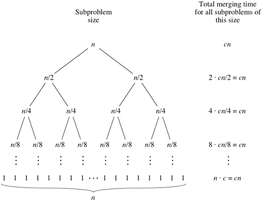
4. There are $\log_2 n + 1$ levels in the tree. +1 because the root level is level 0.
5. The total cost is the sum of the costs at each level, which is $\Theta(n \log_2 n)$.

Exercises

2.3-1

Done with pen and paper.

2.3-2

Assuming the first call to merge_sort(input, p, r), where $r \geq p$, then the test if p != r suffices to ensure that no recursive call has $p > r$. Argument:

• Given that both $p$ and $r$ are both integers and that initially $r \geq p$.
• Also, given the definition of the mean as the balancing point between numbers. We can define the range of the mean for the two possible cases for the inputs:
  • When $p = r$, then the mean (m) is given as: $m = p$.
  • When $r > p$, then the mean (m) is given as: $p < m < r$. Given that we floor the mean to an integer, the true range is: $p \leq m < r$.
• The first possible case for the inputs triggers the if conditional and stops further division.
• The $\lfloor mean(p, r) \rfloor$ of two consecutive $p$ and $q$ integers is $p$.
• This leaves us with two cases for the two recursive merge_sort calls:
  • First recursive call:
    • Case 1 (Consecutive integers): merge_sort(input, p, q). Here, $q = p$, hence, this will trigger the if conditional.
    • Case 2 (Non consecutive integers): merge_sort(input, p, q). Here, $q > p$, thus, the important condition that $r > p$ is maintained.
  • Second recursive call:
    • Case 1 (Consecutive integers): merge_sort(input, q + 1, r). Here, $q = p$, hence, $q + 1 = r$ and this will trigger the if conditional.
    • Case 2 (Non consecutive integers): merge_sort(input, q + 1, r). Here, $r > q + 1$, thus, the important condition that $r > p$ is maintained.

2.3-3

Loop invariant: At the start of each iteration i and j points to the smallest element in the left and right arrays, respectively, that is greater than or equal to the last element in input[p..k-1]. Initialization: At the start of the loop, both i and j are set to 0. Since both arrays are sorted, this is trivially the smallest element. Also, $k = 0$, and the elements in input[p..k-1] is zero. Maintenance: In the loop body, we merge the smallest element between left[i] and right[j] to input[k] and increment i or j (but not both) correspondingly. The k variable is incremented. The loop invariant still holds: input[p..k-1] is still sorted AND left[i] and right[j] are the smallest elements in left and right array that are greater than or equal to the last element of input[p..k-1]. Termination: The loop terminates when all elements of either left or right has been merged.

When the loop terminates, based on the termination condition, either left or right has at least one element that hasn't been merged. The two while loop handles each case (only one case is possible at a time). It merges the leftover elements in the remaining array. Since, both arrays are sorted, the remaining array contains only leftover elements that are greater than any element in the array that was exhausted.

Taken together, the elements in input[p..k-1] represents all the elements in left and right merged together.

2.3-4

TODO

2.3-5

fn insertion_sort_recursive(input: &mut Vec<i32>, r: usize) {
    if (r == 0) {
        return;
    }

    insertion_sort_recursive(input, r-1);
    insert_into_sorted(input, r)
}

fn insert_into_sorted(input: &mut Vec<i32>, r: usize) {
    let mut j = r;
    let current = input[r];
    while (j > 0 && current < input[j - 1]) {
        input[j] = input[j - 1];
        j -= 1;
    }


    input[j] = current;
}

The recurrence relation for the recursive insertion sort is given below: $ T(n) = \begin{cases} \Theta(1) & \text{if } n = 1 \ T(n - 1) + O(n) & \text{if } n > 1 \end{cases} $

The recurrence can be expanded step by step: $ \begin{aligned} T(n) = T(n - 1) + n \ T(n - 1) = T(n - 2) + (n - 1) \ T(n - 2) = T(n - 3) + (n - 2) \end{aligned} $

Adding these terms:

The summation of the first $n$ integers is: $ 1 + 2 + 3 + ... + n = \frac{n(n + 1)}{2} $

Thus, the complexity is still: $ T(n) = \theta(n^2) $

2.3-6

fn binary_search(input: Vec<i32>, p: usize, q: usize, needle: i32) -> Option<usize> {
    if q == p {
        return if input[p] == needle {
            Some(p)
        } else {
            None
        }
    }

    let middle = (p + q) / 2;

    if input[middle] == needle {
        Some(middle)
    } else if input[middle] < needle {
        binary_search(input, middle+1, q, needle)
    } else {
        binary_search(input, p, middle.saturating_sub(1), needle)
    }
}

At each step of the recursion, the problem is halved. This continues until either the element is found early, or the input is left with only one element, and that one element either matches or doesn't (this is the worst case). It takes $log_2 n$ steps to get an $n$ element array to a size of $1$ through repeated halving. Hence, the worst case running time of binary search is $\theta(\log_2 n)$

2.3-7

Using binary search in insertion sort won't improve its runtime. The inner while loop of insertion sort has two responsibilities:

• Find the position to insert the ith element. Binary search can speed this up to $\theta(n \log_2 n)$.
• Swap elements to create room for the ith element to be inserted. Binary search does not help in this domain.

2.3-8

To solve the problem in $\theta(n \log_2 n)$ time, first sort the input with merge sort and then use the procedure below to determine if any element adds up to x in $\theta(n)$ time:

fn sums_up(sorted_input: Vec<i32>, x: i32) -> bool {
    let mut i = 0;
    let mut j = sorted_input.len()-1;

    while (i != j) {
        let sum = sorted_input[i] + sorted_input[j];
        if sum == x {
            return true
        } else if sum > x {
            j -= 1;
        } else {
            i += 1;
        }
    }

    false
}

Problems

2-1 Insertion sort on small arrays in merge sort

a. It takes insertion sort $\theta(n^2)$ time to sort an array on length $n$. If $n = k$ and there are $n / k$ arrays to sort, the total time taken to sort all arrays is $\theta(nk)$.

b. If we apply insertion sort when the elements in merge sort are smaller or equal to $k$, it means we will have $n / k$ leaves, each of size $\leq k$ in the recursion tree of merge sort. This means we will have $log_2 (n / k)$ levels, with a total of $n$ elements per level. This implies it would take us $n \cdot \log_2 (n / k)$ time to merge all nodes in the recursion tree.

c. The modified merge sort with insertion sort runs in $\theta(n \cdot k + n \cdot \log_2 (n/k))$ time. Where $nk$ is the time it takes to perform insertion sort for the bottom nodes. And $n \cdot \log_2 (n / k)$ is the time to merge the top nodes. $k$ must be greater than $1$, else, the running time devolves into the standard merge sort time. But $k$ must also be less than $log_2 (n)$, else, the $nk$ part outgrows the other parts, and the runtime devolves also into the standard merge sort time.

d. $k$ must be in the range specified by (c) above. In practice $k$ can be picked based on empirical tests that depend on the machine, type of data, etc.

2-2 Correctness of bubblesort

TODO

2-3 Correctness of Horner's rule

TODO

2-4 Inversions

a. The five inversions of array [2, 3, 8, 6, 1] are (2, 1), (3, 1), (8, 6), (8, 1), and (6, 1).

b. The array with elements [1, 2, ..., n] that has the most inversions is a reverse sorted array. There are $(n - 1) + (n - 2) + ... + 2 + 1$ inversions in such array which can be calculated with the formula below: $ = \frac{n(n - 1)}{2} $

c. The notion of inversions is strongly related with the inner while loop of insertion sort. The inner while loop is responsible for swapping out of place elements. Each inversion represents an out-of-place element.

d. The merge sort algorithm can be repurposed to count the number of inversions in an array in $\theta(nlog_2 n)$ time:

fn count_inversions(input: &mut Vec<i32>, p: usize, r: usize) -> usize {
    if p >= r {
       return 0;
    }

    let q = (r + p) / 2;
    let mut inversions = count_inversions(input, p, q);
    inversions += count_inversions(input, q + 1, r);
    merge(input, p, q, r, inversions)
}

fn merge(input: &mut Vec<i32>, p: usize, q: usize, r: usize, inversions: usize) -> usize {
    let left_length = (q - p) + 1; // Explanation for the +1: Given that q >= p, there are two cases: when q == p, there is 1 element; and when q > p, e.g. q = 2 and p = 0, there are 3 elements.
    let right_length = (r - q);
    let mut left = vec![0;left_length];
    let mut right = vec![0;right_length];

    for i in 0..left_length {
        left[i] = input[p + i]
    }
    for i in 0..right_length {
        right[i] = input[q + i + 1]
    }

    let mut left_index = 0;
    let mut right_index = 0;
    let mut input_index = p;

    let mut right_inversion_count = inversions;

    while left_index < left_length && right_index < right_length {
        if left[left_index] <= right[right_index] {
            input[input_index] = left[left_index];
            left_index += 1;
        } else {
            input[input_index] = right[right_index];
            right_index += 1;
            right_inversion_count += left_length - left_index;
        }

        input_index += 1;
    }

    while left_index < left_length {
        input[input_index] = left[left_index];
        input_index += 1;
        left_index += 1;
    }

    while right_index <right_length {
        input[input_index] = right[right_index];
        input_index += 1;
        right_index += 1;
    }

    right_inversion_count
}

Chapter 3: Characterizing Running Times

The order of growth of the running time of an algorithm, gives a simple way to characterize the algorithm's efficiency and also allow us to compare it with alternative algorithms.

The precision of an exact running time of an algorithm is rarely worth the effort because for large enough inputs, the multiplicative constants and lower-order terms are dominated by the effects of the input size itself.

The asymptotic efficiency of an algorithm is concerned with how the running time of an algorithm increases with the size of the input in the limit, as the size of the input increases without bound.

Usually, an algorithm that is asymptotically more efficient is the best choice for all but very small inputs.

The three common asymptotic notations

The asymptotic notations described below are designed to characterize functions in general. The function can denote the running time, space usage, etc.

All the functions used in the notation must be asymptotically non-negative. An asymptotically positive function is one that is positive for all sufficiently large $n$.

The goal of the asymptotic notations is to provide a simplified yet precise bound for the running time of an algorithm, so that algorithms can easily be compared.

Big-oh $(O)$ notation

The $O$ notation specifies an asymptotic upper bound on a function to within a constant factor. $O(g(n))$ is pronounced "big-oh of g of n" or just "oh of g of n".

Formal definition

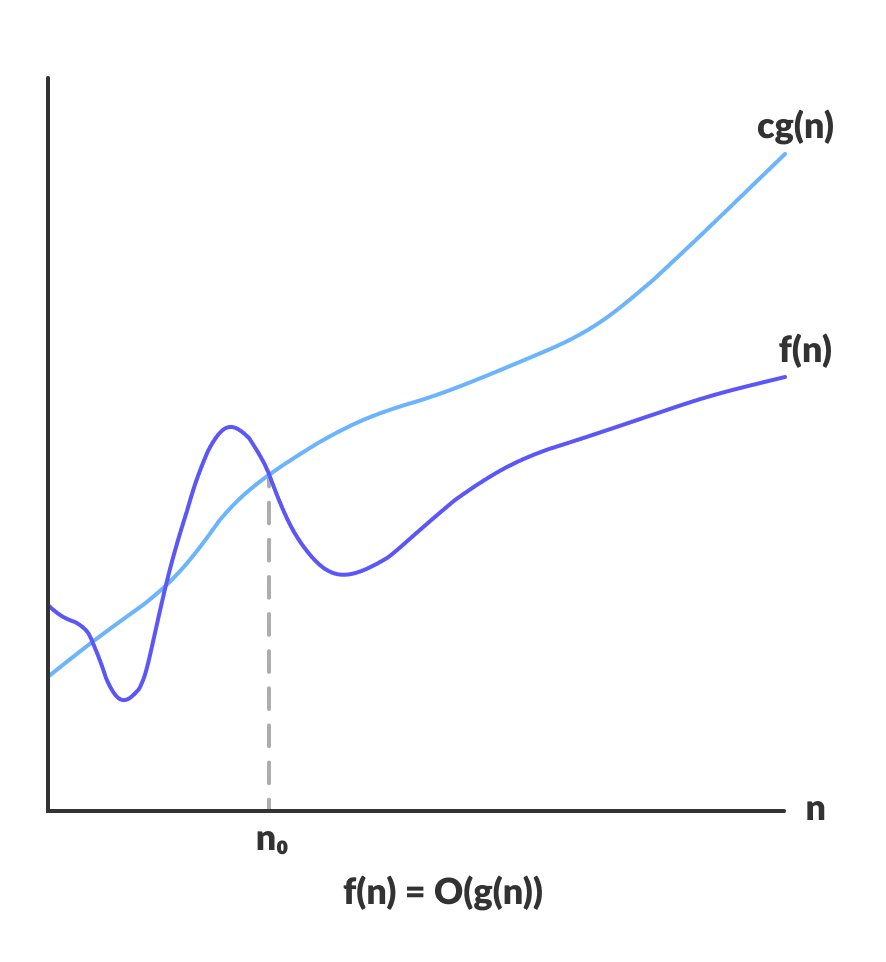
For a given function $g(n)$, we denote by $O(g(n))$ the set of functions:

A function $f(n)$ belongs to the set $O(g(n))$ it there exists positive constants $c$ such that $f(n) \leq c \cdot g(n)$ for sufficiently large $n$.

Example

The example below uses the formal definition to provide justification for the practice of discarding lower-order terms and ignoring the constant coefficient of the highest-order term:

• Given, $f(n) = 4n^2 + 100n + 500$
• We say $f(n) = O(n^2)$
• Because, we can find a $c$ and $n_0$ such that $4n^2 + 100n + 500 \leq c \cdot n^2$
• First simplify the inequality to $4 + 100/n + 500/n^2 \leq c$
• For $n_0 = 1$, then the inequality holds for $c = 604$.
• Or, if $n_0 = 10$, then $c = 19$ works.
• etc

Omega $(\Omega)$ Notation

The $\Omega$ notation provides an asymptotic lower bound. $\Omega(g(n))$ is pronounced "big-omega of g of n" or just "omega of g of n".

Formal definition

For a given function $g(n)$, we denote by $\Omega(g(n))$ the set of functions:

Example

• Given, $f(n) = 4n^2 + 100n + 500$
• We say $f(n) = \Omega(n^2)$
• Because, we can find a $c$ and $n_0$ such that $4n^2 + 100n + 500 \geq c \cdot n^2$
• First simplify the inequality to $4 + 100/n + 500/n^2 \geq c$
• This inequality holds when $n_0$ is any positive integer and $c = 4$.

Theta $(\theta)$ notation

The $\theta$ notation specifies asymptotically tight bounds. $\theta(g(n))$ is pronounced "theta of g of n".

Formal definition

For a given function $g(n)$, we denote by $\theta(g(n))$ the set of functions:

For all $n \geq n_0$, the function $f(n)$ is equal to $g(n)$ to within constant factors.

Theorem

For any two functions, $f(n)$ and $g(n)$,

$f(n) = \theta(g(n))$

IFF

$f(n) = \Omega(g(n))$ and $f(n) = O(g(n))$.

Correctness and precision

The asymptotic notation used to describe an algorithm must be as precise as possible and must correctly state the type of running time it applies to. Examples:

• Correct: Insertion sort has a worst-case running time of $O(n^2)$, $\Omega(n^2)$, and $\theta(n^2)$. The $\theta(n^2)$ bound is the most precise and hence the most preferred.
• Correct: Insertion sort has a best-case running time of $O(n)$, $\Omega(n)$, and $\theta(n)$. The $\theta(n)$ bound is also the most precise and the most preferred.
• Wrong: Insertion sort has a running time of $\theta(n^2)$. This is wrong because without the qualification of "worst-case", the statement covers all running times (best and worst case).
• Correct: We can however say that insertion sort has a running time of $O(n^2)$ because both the best-case and worst-case doesn't grow faster than $n^2$.
• Correct: We can also say that insertion sort has a running time of $\Omega(n)$ because both the best-case and worst-case grows at least as fast as $n$.
• Correct: Merge sort has a running time of $\theta(n \log_2 n)$ because this is true in all cases.

Conflating $O$ with $\theta$

The $O$ notation is occasionally used in scenarios where the $\theta$ notation will be more appropriate. e.g.

• Saying that "an $O(n \lg_2 n)$ time algorithm is faster than an $O(n^2)$ time algorithm".
• This is not necessarily true, because the $O$ notation only specifies an asymptotic upper bound.
• Hence, the $O(n^2)$ might actually run in just $\theta(n)$ time.